Thermal balance, radiators and heaters
Trace a temperature through the Console
Open Sizing and budgets > Thermal. The Symmetric deployable arrays starter shows how a temperature band, node balance and hardware allocation fit together.
Select the case and node
Choose Runtime cold under Design cases. Each row in Node temperature bands is selectable; choose Avionics. Read the temperature marker against the design interval, which includes reserves, as well as the specified limits. Switch to Runtime hot when reviewing the other boundary.
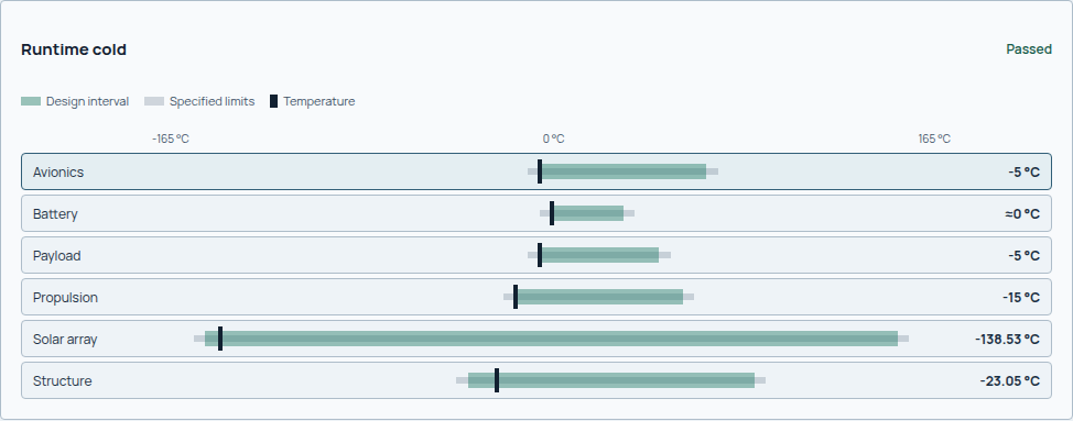
Avionics reaches −5 °C, the lower edge of its design interval. A passing temperature check with approximately zero cold margin has no spare margin beyond the stated reserve. Hot and cold are independent equilibrium cases.
Explain the selected temperature
Read Avionics: heat balance together with Inside avionics. The signed balance separates heat entering and leaving the node; the table distinguishes specified limits, design interval and heater electrical use.
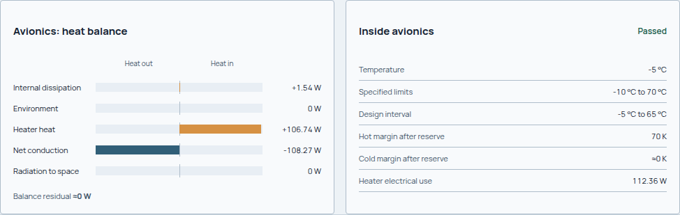
Heater heat contributes 106.74 W while net conduction removes 108.27 W in this case. Heater electrical use is 112.36 W: electrical consumption and heat delivered to the node have different accounting boundaries.
Follow the result into hardware
Continue to Thermal hardware allocations. Compare each radiator's allocated area with its available surface, and each heater's electrical capacity with its node. Inspect in Architecture opens the corresponding allocation. Finish with Thermal sizing checks and Analysis scope and allocation basis.
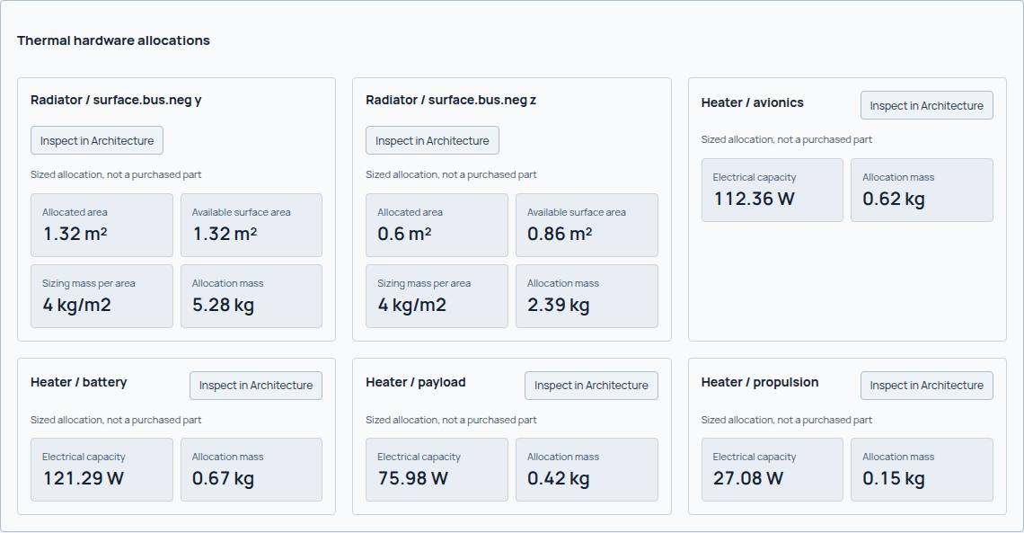
The study allocates 1.92 m² of radiator and 336.71 W of peak heater electrical use. These sized allocations still require hardware design; their cards do not identify purchased radiator or heater assemblies.
What sets the hot and cold cases?
Thermal control must reject heat in the hot case and supply enough heat in the cold case. Sindri estimates equilibrium node temperatures and radiator/heater hardware using internal dissipation, external exposure, conduction and radiation. Read each temperature with its node, geometry state and scenario.
The normal integrated workflow resolves a maintained reference network and
surface mappings from current geometry, power and environment products. It
constructs bounded hot/high-load and cold/low-load cases. Optional design choices
belong in spacecraft.thermal, not mission.thermal. This does not provide an
arbitrary flight network: do not treat a generic node as a particular flight
sensor without a supported mapping.
The hot/cold mode selection excludes heater electrical loads from the initial mode comparison. The cold runtime case removes direct sun/albedo access; the hot case permits it. Both are labelled sustained equilibrium bounds. A recorded duration is not evidence that a transient thermal history was integrated.
Authoring thermal design choices
Use Configure > Subsystems > Thermal, or the same optional thermal section
in spacecraft.yaml. For example:
thermal:
  node_overrides:
    battery:
      minimum_temperature_c: 5.0
      maximum_temperature_c: 40.0
      heater_eligible: true
  bus_finish_id: thermal.finish.az93-white
  margins:
    hot_margin_k: 5.0
    cold_margin_k: 5.0
  installed:
    heater_electrical_power_w: 30.0
Omitted choices inherit the maintained model. Reset in the Console removes an override; it does not write a second copy of the default. CLI and Console use the same validation and solver binding. Limits must form an ordered temperature range after combining overrides with defaults. Unknown nodes, finishes or mode references fail validation rather than silently reverting to defaults.
| Input | Meaning |
|---|---|
node_overrides |
Temperature limits and heater eligibility for maintained nodes; the Console lists their current defaults |
bus_finish_id, array_finish_id, radiator_finish_id |
Compatible entries from the thermal finish catalog; array optical properties do not change EPS cell efficiency |
margins.hot_margin_k, margins.cold_margin_k |
Reserve below maximum and above minimum allowable temperature |
installed.radiator_area_m2, installed.heater_electrical_power_w |
Capacity caps, not imposed demands; zero is a real zero-capacity limit |
hot_case, cold_case |
Optional mode_id, environment_case_id, sun_access_factor and albedo_access_factor selections |
Without explicit case choices, selection retains the automatic hot/high-load and cold/low-load bounds. An authored mode carries its existing geometry state and scenario binding; it does not create an independent thermal timeline. Environment case IDs are checked against the generated environment product when solving. Access factors lie between 0 and 1 and default to 1 for hot and 0 for cold.
User-entered temperature limits are design assumptions, not verified hardware
ratings. A node override may cite a source_id declared in the spacecraft's
evidence_sources; otherwise its limits are attributed to the project input.
Changing inputs changes the sizing calculation and its cache identity, not just
the report. Installed limits can therefore produce explicit failed assessments.
Node heat balance
The diagram shows the terms for a generic node in the equilibrium model. It is an explanation of the heat balance, not a mission-specific thermal network.
flowchart TD
    accTitle: Heat paths in an equilibrium node
    accDescr: Internal dissipation, absorbed external heat and heater power enter a thermal node. Conductive exchange connects neighboring nodes, and radiation connects the node to its space sink. The steady-state solver balances these terms.
    INTERNAL["Internal dissipation"] --> NODE["Node temperature"]
    EXTERNAL["Absorbed external heat"] --> NODE
    HEATER["Heater heat"] --> NODE
    OTHER["Neighboring nodes"] <-->|"Conductive exchange"| NODE
    NODE -->|"Radiation"| SPACE["Space sink"]
For each node at equilibrium:
\(G_{ij}\) couples node \(i\) to node \(j\) by conduction; \(K_{i,\mathrm{rad}}\) is node \(i\)'s radiation coefficient.
Heat terms are in W, conductance in W/K, temperatures in K for the equation, and radiation coefficient in W/K⁴. It incorporates emitting area, emissivity, view treatment and the Stefan–Boltzmann constant. Reported temperatures may be in °C; never raise a Celsius temperature to the fourth power in this balance.
Surface absorptivity/emissivity and area govern external absorption and radiative loss. Geometry supplies source exposure; thermal supplies optical properties and flux-to-heat conversion. Internal electrical demand and dissipated heat must retain their correct boundaries.
The nonlinear network solve uses safeguarded node roots and damping. It checks heat residual and temperature change, and reports invalid/no-sink networks or non-convergence as failures. A converged equilibrium can still violate allowable node temperatures.
Sizing and system feedback
Radiator allocation is bounded by eligible physical surfaces and selected surface treatments. An unconstrained theoretical radiator area is not available spacecraft area. Review allocation, total area, area margin and remaining hot-case temperature violations.
Heater sizing solves for local heat at each eligible node's cold design target, bounded by heater capacity. Heat at a node decreases when conduction from another node supplies it. For cold nodes without heaters, a bounded deterministic search raises eligible targets while respecting every node's upper design limit. This conductive fallback is not a general optimizer: failure means no allocation was found within its bounds. Networks with disconnected nodes lacking any radiative sink are rejected. A successful heater allocation must meet both temperature bounds; capacity or conflicting limits remain explicit failures.
Installed electrical capacity is the sum of per-node peak allocations across scenarios; operating demand is each scenario's delivered heat divided by heater efficiency. EPS carries the controlling demand for each mode and node throughout that mode, including sunlight and eclipse, as a conservative sustained cold bound. The result labels this assumption; the model cannot infer thermostat duty or turn heaters off in sunlight. The network receives heater heat explicitly without counting its EPS feedback twice. Hardware also enters mass.
| Evidence | Read it for |
|---|---|
| Scenario and node balances | Temperature, external/internal/heater heat, conduction, radiation and residual |
| Surface heat records | Finish, exposure, source and absorbed heat assumptions |
| Hardware allocations | Radiator area, heater power, mass and supported placement |
| Assessment/applicability | Temperature violations, unsupported claims and degraded assumptions |
Limits and interpretation
The represented solution is steady state. It does not predict thermal settling time, orbital temperature oscillations, detailed transient battery behavior or thermal-vacuum qualification. Material/finish assumptions and generic network conductances need evidence before a mission-specific comparison is credible.
EX02 and EX03 show how heater power and radiator allocation appear alongside warnings or failed coupled assessments. A zero reported radiator area does not cancel a failed thermal assessment, as the topology comparison demonstrates.
Read the thermal result reference with power and geometry, preserving scenario/state identity when comparing outputs.