Electrical power and energy storage
Follow a mode from generation to hardware
Choose Sizing and budgets > Power in a completed run. This walkthrough uses the Symmetric deployable arrays starter and compares Payload / Sunlight with Downlink / Eclipse. These are two different operating cases, with different loads as well as different environments.
Compare sunlight and eclipse
Under Operating modes, select Payload, then Sunlight under Environment. Read Power balance against its legend: available generation and generation actually delivered to the bus are separate quantities. Mode time allocation supplies the duration context.
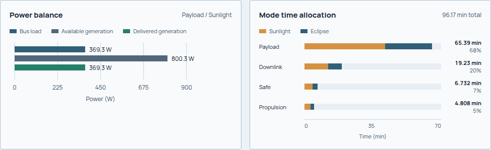
Read the Payload case's load and generation together. The accompanying durations give its share of the sizing cycle; these are recorded sizing cases, not a plot of orbital event times.
Now select Downlink, then Eclipse. This case has its own operating load and zero solar generation. Follow the battery contribution before interpreting zero generation as an unserved load.
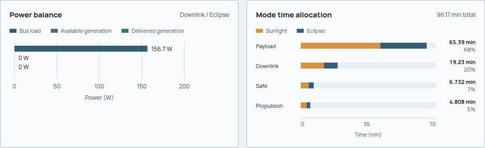
This case supplies 156.7 W of bus load from the battery. Its recorded unserved load is 0 W; the battery, rather than the array, is serving this segment.
Read the segment's energy and load terms
Continue to Inside the mode. The table distinguishes battery bus power in W from battery energy change in Wh. Use What drives the load? to identify the subsystems behind the demand, including bus-side losses and reserves.
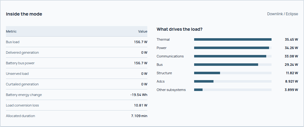
The captured eclipse allocation lasts 7.109 min and records a −19.54 Wh battery energy change. A power value and an energy change answer different questions.
Check the hardware and the whole cycle
Read Required and installed, then Overall sizing checks. Compare the array's required, installed and realized areas; compare storage against usable end-of-life energy. Inspect controlling case returns a cycle/storage check to its driving segment. Explore EPS architecture opens the hardware behind it.
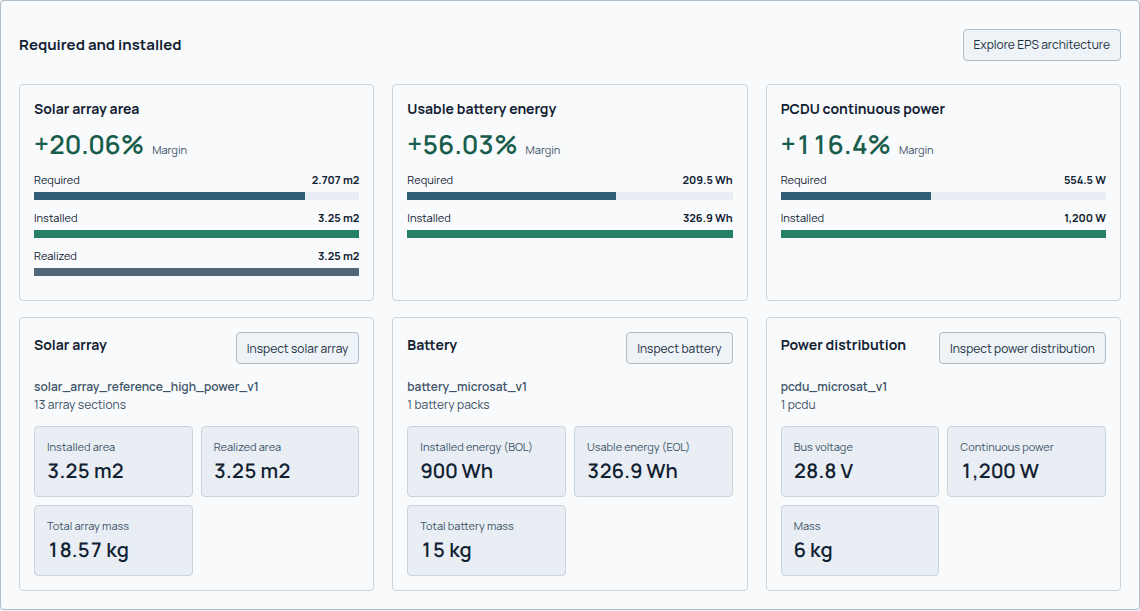
The recorded array uses 3.25 m² against 2.707 m² required; usable battery energy is 326.9 Wh against 209.5 Wh required. Individual positive margins coexist with the overall Review needed state. Review the recorded checks and applicability before accepting the design.
Can the spacecraft supply its loads throughout the cycle?
A power design must meet loads when they occur and replenish the battery over the operating cycle. Start with the timeline and load ledger, then check the array, battery and power-conditioning hardware that must deliver that energy.
Author EPS hardware/technology choices, bus voltage (V), efficiencies, degradation case and a chronological timeline of modes, durations (s) and sunlight/eclipse states. Modes reference the same payload, communications and propulsion activity used elsewhere. Choose a supported timeline template or an explicit cycle; clear the template selection when supplying the full explicit timeline. See mission fields.
The load ledger distinguishes component states, subsystem contributions, conversion losses, reserve and heater demand. RF transmit output in W is not transmitter electrical consumption. Read the resolved bus-load terms rather than adding headline powers without their states and efficiency boundaries.
Generation and hardware
The generation ledger combines represented solar exposure with panel response, conversion/availability factors and lifetime retention. For a sunlight segment:
Delivered power density \(p_{\mathrm{delivered}}\) is in W/m² and array area \(A_{\mathrm{array}}\) in m², giving available generation \(P_{\mathrm{gen}}\) in W.
Eclipse generation is zero in this calculation. Geometry has already projected and occluded the relevant surfaces; do not apply incidence again. Required array area and realized array area answer different questions. The physical embodiment must actually provide usable area under the bound attitudes.
Hardware resolution checks array electrical configuration, battery packs and power-conditioning compatibility. Installed BOL energy, usable EOL energy, voltage/current capability, depth-of-discharge limits and total hardware mass are distinct outputs. A reported convergence scalar does not replace a valid resolved EPS architecture.
Chronological battery balance
Follow the balance at the bus before applying battery efficiency. The diagram shows the sign convention used in the equations; actual storage and delivery limits are checked in the segment evaluation.
flowchart TD
    accTitle: Battery charge and discharge balance
    accDescr: Compare available generation with load. A deficit discharges the battery through discharge efficiency; a surplus charges it through charge efficiency. Energy changes over the segment duration. Empty storage leaves unserved load and full storage can curtail generation.
    SIGN["Load minus available generation"]
    SIGN -- "Positive: deficit" --> DISCHARGE["Discharge through battery efficiency"]
    SIGN -- "Negative: surplus" --> CHARGE["Charge through battery efficiency"]
    DISCHARGE --> ENERGY["Update energy and check storage limits"]
    CHARGE --> ENERGY
For each segment, positive battery bus power means discharge:
The efficiencies \(\eta_{\mathrm{charge}}\) and \(\eta_{\mathrm{discharge}}\) are dimensionless. With terminal power in W and segment duration \(\Delta t\) in s, \(\Delta E\) is in Wh; charging increases stored energy.
Storage sizing evaluates the cyclic drawdown across the timeline seam as well as net cycle energy. A battery can bridge an eclipse yet fail to recharge over a complete cycle. The bounded timeline evaluation records beginning/end energy, curtailed generation when full, and unserved load when empty. Nonnegative stored energy produced by clipping is not proof that all loads were served.
Review recharge margin, required usable energy, available storage margin, controlling segment and every unserved-load term. Chronology matters: equal daily generation and consumption do not imply adequate capacity at every point.
Recorded energy fields
The power method records two related calculations in
PowerResultPayloadV2. Both use W, seconds and Wh, with battery charge/discharge
efficiencies applied at the terminal boundary shown above.
| Field | Definition and scope |
|---|---|
energy_sizing.net_cycle_energy_wh |
Sum of unconstrained terminal energy increments over the complete authored timeline, using available generation and requested load before capacity clipping. |
energy_sizing.recharge_margin_wh |
Equal to net_cycle_energy_wh; assesses full-cycle recharge against the EPS energy-balance tolerance. |
energy_sizing.required_usable_energy_wh |
Maximum cyclic storage drawdown, including the timeline seam, in Wh. |
energy_sizing.controlling_segment_id |
Segment ending the controlling storage drawdown after rotation to the maximum-energy boundary. It identifies the capacity driver, while recharge includes all segments. |
margins[] with metric_id: eps.margin.usable-storage |
Available usable battery energy minus energy_sizing.required_usable_energy_wh, in Wh. A negative margin records a storage shortfall. Available usable energy can use a retained fallback when architecture resolution fails. |
segments[].battery_energy_delta_wh |
Bounded stored-energy change for that segment after delivery/storage limits; equals end energy minus start energy. |
segments[].curtailed_generation_w |
Available generation not delivered because it cannot be used or stored. |
segments[].unserved_load_w |
Requested bus load not supplied by delivered generation and battery discharge. |
required_solar_array_area_m2 |
Continuous sizing requirement or retained diagnostic bound when no finite solution exists; interpret with sizing status and issues. |
realized_solar_array_area_m2 |
Realized area used by the generation calculation. |
architecture.array.installed_area_m2 |
Area of the resolved selected array hardware; unavailable when no architecture was resolved. |
Summing bounded segment storage changes can differ from the unconstrained sizing balance because of curtailment and unserved loads. A full-cycle energy balance and an individual segment's storage change therefore have different scopes. These definitions apply to the recorded calculation horizon; different mode dwell times or mission schedules require corresponding evidence.
Thermal and lifetime coupling
flowchart TD
    accTitle: Electrical power feedback with thermal and lifetime sizing
    accDescr: Geometry provides exposure and lifetime provides retained capability to electrical sizing. Electrical dissipation feeds thermal sizing, heater demand returns to power, and both models update hardware, mass and geometry for the next iteration.
    EXPOSURE["Geometry and environmental exposure"] --> EPS["Power generation and battery balance"]
    LIFE["Lifetime retention"] --> EPS
    EPS -- "Electrical dissipation" --> THERMAL["Thermal temperatures and hardware"]
    THERMAL -- "Heater electrical demand" --> EPS
    EPS --> HARDWARE["Hardware mass and geometry"]
    THERMAL --> HARDWARE
    HARDWARE -. "Next iteration" .-> EXPOSURE
Thermal sizing returns mode-specific heater electrical demand, which is fed back
into EPS. Heater energy can control storage or generation even when payload
average power is modest. eps.heater.sustained-cold-bound identifies demand
applied throughout the affected mode in sunlight and eclipse. It is a conservative
bound from equilibrium sizing, not installed capacity or predicted thermostat
duty. Array/battery retention reduces capability over the
design life; see lifetime. Hardware mass and geometry then return
to the integrated sizing loop.
Each new placement pass retains the preceding thermal demand and physical array realization for storage sizing. Geometry receives the selected whole-section array area; continuous required area remains separately reported. These discrete hardware sizes are not damped to fractional sections or packs. Convergence also checks for hardware changes after placement. Generation always uses realized area, so unplaced panels and insufficient mounting space remain visible failures. When no feasible EPS chain exists, the energy ledger uses retained physical battery capacity where available; it cannot invent extra packs outside the mass and placement ledger. Storage deficits and unserved loads remain visible.
The current power result marks failed hardware/energy constraints as fail;
otherwise it retains a warning with degraded model applicability. That warning
is part of the result, not permission to describe the design as qualified.
Failures and limits
eps.array-sizing.no-finite-cycle-recharge means the resolved exposure and
loads cannot close the authored cycle by increasing array area. Sindri retains
a bounded state for continued diagnosis; that area is not a feasible solution.
Review orientation, exposure, load scheduling and architecture before rerunning.
EX01 and EX04
show this condition.
EX02 also illustrates why a zero battery scalar beside a failed EPS assessment is not a zero-storage recommendation. Inspect architecture availability and candidate rejection reasons first.
The model is a preliminary hardware/energy calculation, not a detailed switching simulation, electrochemical qualification or proven flight power service.
Panel Mass And Area
EPS owns panel assembly mass. Its recorded basis includes substrate, photovoltaics and panel wiring, but not deployment mechanisms or separate mounting brackets. Catalog assembly masses are not stretched to arbitrary panel geometry. Estimated custom panels use the selected catalog areal mass times physical gross area.
Electrical section area and physical area are different. Deployment converts the section-rounded electrical target to active cell area using the selected reference packing factor. Panel geometry then adds its own inactive packing area and borders. Power uses active area divided by reference packing; mass includes the borders. For example, nine 0.25 m2 sections at 0.94 reference packing require 2.115 m2 cells. Two square leaves at 0.90 packing with 20 mm borders occupy 2.526636 m2, giving 12.633179 kg at 5 kg/m2, before separate mechanisms. Unrepresented electrical sections are a failed realization, not invisible hardware in the bus.
The generic 5 kg/m2 panel-only estimate is consistent with the construction range in the Rocket Lab STARRAY sheet (L-Star 3.3; T-Star 4.3-5.8 kg/m2). This is a scope/plausibility check, not calibration of every catalog panel or deployment mechanism. Older class archetypes retain their recorded, uncalibrated densities; select a suitable evidenced component. The legacy 2.8 kg/m2 power constant no longer drives deployed panel mass. Historic results without a mass basis remain unrecorded, not retroactively verified. An electrically infeasible result can still retain known installed hardware mass. Realized panel borders remain included, and the catalog construction method is not replaced merely because cycle recharge fails. That retained mass is not an assertion that the array supplies sufficient power.
Use the power result reference for exact ledgers, segments and assessment fields.